San Diego Tracts#
This dataset contains an extract of a set of variables from the 2017 ACS Census Tracts for the San Diego (CA) metropolitan area.
import contextily
import geopandas
import cenpy

acs = cenpy.products.ACS(2017)
Download Data#
Set variables to download
vars_to_download = {
    "B25077_001E": "median_house_value",  # Median house value
    "B02001_002E": "total_pop_white",     # Total white population
    "B01003_001E": "total_pop",           # Total population
    "B25003_003E": "total_rented",        # Total rented occupied
    "B25001_001E": "total_housing_units", # Total housing units
    "B09019_006E": "hh_female",           # Female households
    "B09019_001E": "hh_total",            # Total households
    "B15003_002E": "total_bachelor",      # Total w/ Bachelor degree
    "B25018_001E": "median_no_rooms",     # Median number of rooms
    "B19083_001E": "income_gini",         # Gini index of income inequality
    "B01002_001E": "median_age",          # Median age
    "B08303_001E": "tt_work",              # Aggregate travel time to work
    "B19013_001E": "median_hh_income"     # Median household income
}
vars_to_download_l = list(vars_to_download.keys())
Download geometries and attributes
%%time
db = acs.from_msa("San Diego, CA",
                  level="tract",
                  variables=vars_to_download_l
                 )
/opt/conda/lib/python3.7/site-packages/pyproj/crs/crs.py:53: FutureWarning: '+init=<authority>:<code>' syntax is deprecated. '<authority>:<code>' is the preferred initialization method. When making the change, be mindful of axis order changes: https://pyproj4.github.io/pyproj/stable/gotchas.html#axis-order-changes-in-proj-6
  return _prepare_from_string(" ".join(pjargs))
CPU times: user 1.12 s, sys: 153 ms, total: 1.27 s
Wall time: 30.8 s
Metadata#
We will also write a companion file with the names of each variable:
var_names = acs.variables\
               .reindex(vars_to_download)\
               [["label", "concept"]]\
               .reset_index()\
               .rename(columns={"index": "var_id"})
var_names["short_name"] = var_names["var_id"].map(vars_to_download)
Process data#
While the ACS comes with a large number of attributes, we are not limited to the original variables at hand; we can construct additional variables. This is particularly useful when we want to compare areas that are not very similar in some structural characteristic, such as area or population. For example, a quick look into the variable names shows most variables are counts. For tracts of different sizes, these variables will mainly reflect their overall population, rather than provide direct information about the variables itself. To get around this, we will cast many of these count variables to rates, and use them in addition to a subset of the original variables.
Replace missing values with columns mean
filler = lambda col: col.fillna(col.mean())
db.loc[:, vars_to_download] = db.loc[:, vars_to_download]\
                                .apply(filler)
Replace variable codes with short names
db = db.rename(columns=vars_to_download)
Calculate area in Sq.Km (we use the Conus Albers CRS)
db["area_sqm"] = db.to_crs(epsg=5070).area / 1e6
Percentage of renter occupied units
db["pct_rented"] = db["total_rented"] / \
                  (db["total_housing_units"] + \
                   (db["total_housing_units"]==0) * 1
                  )
Percentage of female households
db["pct_hh_female"] = db["hh_female"] / \
                  (db["hh_total"] + \
                   (db["hh_total"]==0) * 1
                  )
Percentage with a Bachelor’s degree
db["pct_bachelor"] = db["total_bachelor"] / \
                  (db["total_pop"] + \
                   (db["total_pop"]==0) * 1
                  )
Percentage of white population
db["pct_white"] = db["total_pop_white"] / \
                  (db["total_pop"] + \
                   (db["total_pop"]==0) * 1
                  )
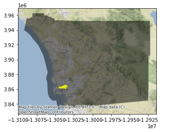
Generate indicator for subset of contiguous 30 tracts
tract_geoids = [
     '06073000100',
     '06073000201',
     '06073000202',
     '06073000300',
     '06073000400',
     '06073000500',
     '06073000600',
     '06073000700',
     '06073000800',
     '06073000900',
     '06073001000',
     '06073001100',
     '06073001200',
     '06073001300',
     '06073001400',
     '06073001500',
     '06073001600',
     '06073001700',
     '06073001800',
     '06073001900',
     '06073002001',
     '06073002002',
     '06073002100',
     '06073002201',
     '06073002202',
     '06073002301',
     '06073002302',
     '06073002401',
     '06073002402',
     '06073002501'
]
db["sub_30"] = False
db.loc[db["GEOID"].isin(tract_geoids), "sub_30"] = True
ax = db.plot(alpha=0.5, color="k")
db[db["sub_30"]].plot(ax=ax, color="yellow")
contextily.add_basemap(ax, crs=db.crs);

Write Out#
db.info()
<class 'geopandas.geodataframe.GeoDataFrame'>
Int64Index: 628 entries, 0 to 627
Data columns (total 25 columns):
 #   Column               Non-Null Count  Dtype
---  ------               --------------  -----
 0   GEOID                628 non-null    object
 1   geometry             628 non-null    geometry
 2   median_age           628 non-null    float64
 3   total_pop            628 non-null    float64
 4   total_pop_white      628 non-null    float64
 5   tt_work              628 non-null    float64
 6   hh_total             628 non-null    float64
 7   hh_female            628 non-null    float64
 8   total_bachelor       628 non-null    float64
 9   median_hh_income     628 non-null    float64
 10  income_gini          628 non-null    float64
 11  total_housing_units  628 non-null    float64
 12  total_rented         628 non-null    float64
 13  median_no_rooms      628 non-null    float64
 14  median_house_value   628 non-null    float64
 15  NAME                 628 non-null    object
 16  state                628 non-null    object
 17  county               628 non-null    object
 18  tract                628 non-null    object
 19  area_sqm             628 non-null    float64
 20  pct_rented           628 non-null    float64
 21  pct_hh_female        628 non-null    float64
 22  pct_bachelor         628 non-null    float64
 23  pct_white            628 non-null    float64
 24  sub_30               628 non-null    bool
dtypes: bool(1), float64(18), geometry(1), object(5)
memory usage: 123.3+ KB
Dataset
! rm -f sandiego_tracts.gpkg
db.to_file("sandiego_tracts.gpkg", driver="GPKG")
Metadata
! rm -f sandiego_tracts_varnames.json
var_names.to_json("sandiego_tracts_varnames.json")


