H3 Grid

Build a H3 grid for the San Diego region

H3 grid

This dataset contains a hexagonal tesselation following Uber’s H3 system that covers the core of San Diego.

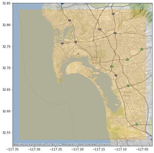
The delineation of the city centre is somewhat arbitrary, was manually drawn using geojson.io, and is stored in sd_city_centre.geojson in this folder.

• Source: Uber

• URL

https://eng.uber.com/h3/

• Processing: Generation of the dataset is documented in build_nasadem_sd.ipynb

Infrastructure

To create a container that includes h3 save the following on a file called Dockerfile:

FROM darribas/gds_dev:4.1

USER root
RUN wget -O - https://apt.kitware.com/keys/kitware-archive-latest.asc 2>/dev/null | sudo apt-key add - \
 && apt-add-repository 'deb https://apt.kitware.com/ubuntu/ bionic main' \
 && apt-get update \
 && apt-get install --yes cmake
USER $NB_UID
RUN pip install h3

And build the container by running the following from the same folder where the file is stored:

docker build -t gds_h3 .

When if finishes, you should be able to launch the gds_h3 container and run this notebook from there.

%matplotlib inline

from h3 import h3
import geopandas
from shapely.geometry import Polygon
import contextily as ctx
import cenpy

Region to cover

sd = geopandas.read_file("sd_city_centre.geojson")
ax = sd.plot(alpha=0.25, color="orange", figsize=(9, 9))
ctx.add_basemap(ax, crs=sd.crs.to_string())

Build H3 geography

%time hexs = h3.polyfill(sd.geometry[0].__geo_interface__, 8, geo_json_conformant = True)

CPU times: user 8.19 ms, sys: 861 µs, total: 9.05 ms
Wall time: 10 ms

polygonise = lambda hex_id: Polygon(
                                h3.h3_to_geo_boundary(
                                    hex_id, geo_json=True)
                                    )

%time all_polys = geopandas.GeoSeries(list(map(polygonise, hexs)), \
                                      index=hexs, \
                                      crs="EPSG:4326" \
                                     )

CPU times: user 101 ms, sys: 7.66 ms, total: 109 ms
Wall time: 109 ms

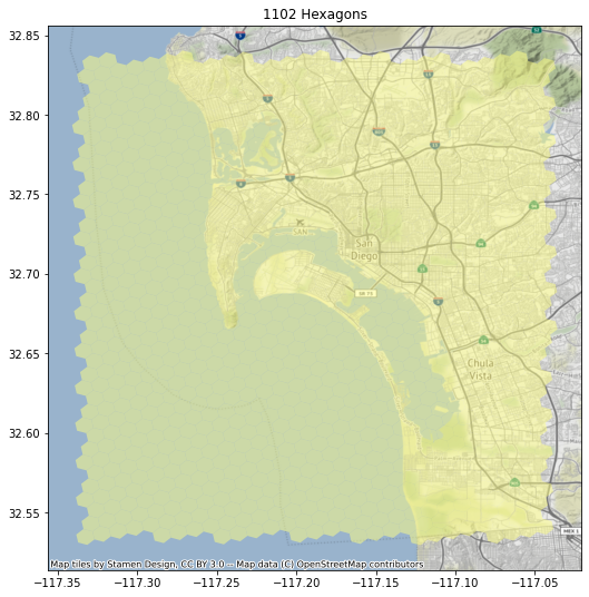
ax = all_polys.plot(alpha=0.5, color="xkcd:pale yellow", figsize=(9, 9))
ctx.add_basemap(ax, crs=all_polys.crs.to_string())
ax.set_title(f"{all_polys.shape[0]} Hexagons");

Clip ocean out

There are quite a few hexagons that fall within the ocean. Let’s get rid of them. For that, we will pull down the polygon for San Diego county using cenpy:

census = cenpy.Decennial2010()
tracts = census.from_msa("San Diego, CA", level="tract")

/opt/conda/lib/python3.7/site-packages/pyproj/crs/crs.py:55: FutureWarning: '+init=<authority>:<code>' syntax is deprecated. '<authority>:<code>' is the preferred initialization method. When making the change, be mindful of axis order changes: https://pyproj4.github.io/pyproj/stable/gotchas.html#axis-order-changes-in-proj-6
  return _prepare_from_string(" ".join(pjargs))
/opt/conda/lib/python3.7/site-packages/pyproj/crs/crs.py:55: FutureWarning: '+init=<authority>:<code>' syntax is deprecated. '<authority>:<code>' is the preferred initialization method. When making the change, be mindful of axis order changes: https://pyproj4.github.io/pyproj/stable/gotchas.html#axis-order-changes-in-proj-6
  return _prepare_from_string(" ".join(pjargs))

Now these geometries include also some ocean:

ax = tracts.plot(alpha=0.5, color="xkcd:pale green")
ctx.add_basemap(ax, crs=tracts.crs.to_string())

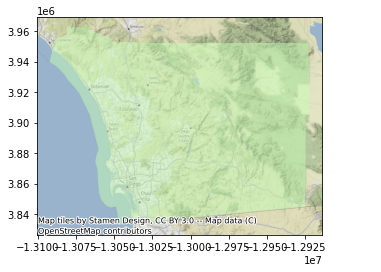
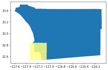
It turns out that part is a separate polygon that may be removed easily:

tracts.head()

	GEOID	geometry	NAME	state	county	tract
0	06073018200	POLYGON ((-13066573.290 3920769.610, -13066530...	Census Tract 182, San Diego County, California	06	073	018200
1	06073018601	POLYGON ((-13067719.770 3922939.420, -13067631...	Census Tract 186.01, San Diego County, California	06	073	018601
2	06073018000	POLYGON ((-13064524.900 3917063.650, -13064338...	Census Tract 180, San Diego County, California	06	073	018000
3	06073017900	POLYGON ((-13064042.110 3917657.290, -13064035...	Census Tract 179, San Diego County, California	06	073	017900
4	06073018510	POLYGON ((-13064367.720 3923018.450, -13064295...	Census Tract 185.10, San Diego County, California	06	073	018510

tracts_land_one = geopandas.GeoDataFrame(
                        {"geometry": [tracts.query("GEOID != '06073990100'").unary_union],
                         "id": ["one"]
                        }, crs=tracts.crs)

ax = tracts_land_one.to_crs(epsg=4269).plot()
all_polys.to_crs(epsg=4269).plot(color="xkcd:pale yellow", ax=ax)

<matplotlib.axes._subplots.AxesSubplot at 0x7fdbf6eeb090>

Let’s convert all_polys into a GeoDataFrame:

h3_all = geopandas.GeoDataFrame({"geometry": all_polys,
                                 "hex_id": all_polys.index},
                                crs=all_polys.crs
                               )

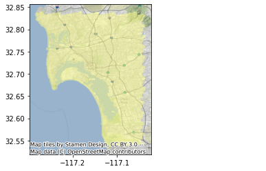
We’re an overlay away from our target:

%%time
h3_land = geopandas.overlay(h3_all, 
                            tracts_land_one.to_crs(h3_all.crs), 
                            how="intersection"
                           )

CPU times: user 3.43 s, sys: 43 ms, total: 3.47 s
Wall time: 3.46 s

ax = h3_land.plot(alpha=0.5, color="xkcd:pale yellow")
ctx.add_basemap(ax, crs=h3_land.crs.to_string())

Write out to GPKG

! rm sd_h3_grid.gpkg
h3_land.drop("id", axis=1).to_file("sd_h3_grid.gpkg", driver="GPKG")

Tract Vs H3 geographies

Get tracts only within the grid:

shp = geopandas.GeoDataFrame(
    {"geometry": [h3_land.unary_union],
     "id": ["one"]
    }, crs = h3_land.crs).to_crs(tracts.crs)
sub = geopandas.overlay(tracts, shp, how="intersection")

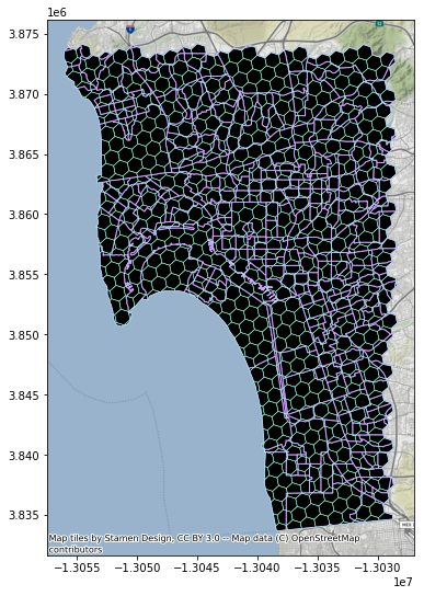
Compare:

ax = sub.plot(facecolor="k", edgecolor="xkcd:lilac", figsize=(9, 9))
h3_land.to_crs(sub.crs).plot(facecolor="none", linewidth=0.5, edgecolor="xkcd:light aqua", ax=ax)
ctx.add_basemap(ax, crs=sub.crs.to_string())

---

Download link

[Download the *sd_h3_grid.gpkg* file]